Statistical Hypothesis Testing Made Simple
Dive into the world of hypothesis testing, where data tells its own story. In this blog, I will try to simplify this statistical method with a courtroom analogy, apply it to a coin toss, and then use it to solve a practical problem: identifying temperature units in time series data.
Understanding Statistical Hypothesis Testing: A Courtroom Analogy
In this section, I will try to explain what hypothesis testing is by taking analogies from a courtroom. I promise you that after you have finished reading this section you will no longer ever hesitate to use hypothesis testing as a method for statistical inference. So, imagine for a couple of minutes that you are sitting as a judge in a courtroom.
The Presumption of Innocence: The Null Hypothesis
Hypothesis testing is the process where data is put on trial, and it’s up to you to judge its story. Every trial begins with the presumption of innocence, and in the world of hypothesis testing, this is known as the null hypothesis. It’s the default position that there is no change, no effect, or no difference. Opposing the null hypothesis is the alternative hypothesis, which holds that there is indeed an effect or a difference.
The Trial: Testing the Data
As the judge, you’re presented with evidence. In hypothesis testing, the evidence is the data itself. You examine it carefully, looking for signs that might contradict the null hypothesis. Is the data too unusual to be just a random chance? Or does it fall within the expected range of variability? In the process of looking for signs, you apply statistical calculations called statistical tests. These calculations measure how far the data deviates from what the null hypothesis would predict. If the deviation is small, you lean toward innocence; if it’s large, toward guilt.
The Verdict: Rejecting the Null Hypothesis or Favoring the Alternative
After careful consideration, you must reach a verdict. If the evidence – the data – is not strong enough to reject the null hypothesis, you maintain the status quo. However, if the data is significantly different from what was expected under the null hypothesis, you reject it, accepting the alternative hypothesis. Caution needs to be taken in interpreting the results of this process. Rejecting or accepting a hypothesis does not mean that the hypothesis is true or not. In statistical inference, we can never prove the truthfulness of a hypothesis based on a sample of data; it is only possible to disprove a hypothesis based on evidence. This also implies that rejecting the null hypothesis doesn’t implicitly mean accepting the alternative. It just means that the evidence favors the alternative hypothesis; again we can’t prove a hypothesis solely on statistical inference. This is probably why this statistical method is called statistical hypothesis testing; we test a hypothesis for its robustness in the face of evidence.
Understanding Statistical Hypothesis Testing: The Case of a Fair Coin
Now, that you understand the idea behind hypothesis testing, let’s apply it to the case of inspecting whether a coin we have borrowed from a friend is fair. First, we have to establish our hypotheses:
- Null Hypothesis: The coin is fair, meaning there is an equal chance of landing heads or tails, i.e.,
- Alternative Hypothesis: The coin is not fair, and the probability of heads or tails is not equal, i.e.,
This type of hypothesis is called a two-sided hypothesis. We would have a right-tailed or left-tailed hypothesis if
\[H_0: p<=1/2, \, H_a: p>1/2\]or
\[H_0: p>=1/2, \, H_a: p<1/2\]holds, respectively. For our coin case, this would translate into questioning whether our coin is biased toward heads or tails, respectively. In our example here, we are interested in whether it is biased regardless of which side of the coin occurs more often.
Next, to test these hypotheses, we conduct an experiment by flipping the coin a certain number of times, say 100, and recording the outcomes. Suppose that we observe that our coin landed 60 times on heads and 40 times on tails (the specific order of events – heads or tails – is irrelevant to this null hypothesis). Is this result due to random chance, or is it evidence of an unfair coin?
To answer this question, we have to choose a statistical test and apply it to the experiment. During the course of mathematical history, many tests have been designed to address specific types of hypotheses, the various experimental scenarios, and the assumptions being made about the samples, e.g., Z-test, T-test, Chi-squared test, etc. The outcome of such a test is a test statistic, that quantifies how far our observed result (60 heads) is from the expected result under the null hypothesis (50 heads). For a coin toss, we might use a test like the chi-square or binomial test. Equivalently to the test statistic, we can calculate the p-value, which is the probability of observing a result as extreme as, or more extreme than, the one we obtained (60 heads or more), assuming the null hypothesis is true.
Before we calculate the p-value, we need to set a threshold for how extreme the results must be to reject the null hypothesis. This threshold is called the significance level, often denoted as \(\alpha\). A common choice for \(\alpha\) is 0.05, which means there is a 5% chance of rejecting the null hypothesis when it is actually true – type I error. Why bother setting a significance level in the first place? Well, it is considered good scientific practice to set the significance level before conducting a test, as doing it after the test would result in a loss of objectivity due to the direct subjective involvement of the researcher in drawing the conclusion from the experiment. If the p-value is less than or equal to our significance level, we reject the null hypothesis. If it’s greater, we do not have enough evidence to reject it.
Let’s calculate what is the p-value for our experiment if we want to test the two-sided hypothesis of the coin being fair using the binomial test. For a sample size \(n=100\), number of heads \(k=60\), we expect under the null hypothesis \(p=1/2\) an equal amount of heads and tails. The probability of our observed number of heads is
\[\mathrm{Pr}(X=k)={n \choose k} p^k\left(1-p\right)^{n-k} \approx 0.01\]In order to calculate the p-value we have to consider all possible outcomes as, or more, extreme than the one we observed. Hence for \(k\geq60\) and \(k\leq40\) we get for our p-value
\[p=\sum_{i=60}^{100}{\mathrm{Pr}(X=i)} + \sum_{i=0}^{40}{\mathrm{Pr}(X=i)} \approx 0.056\]Since \(\alpha=0.05\) we can’t reject the null hypothesis in favor of the alternative at this significance level. Hence, we must further assume that the coin is fair. With this choice, there might be a chance that we are making a wrong judgment about the coin leading to a so-called type II error, i.e., the null hypothesis is false; the coin is actually biased. Let’s say our p-value was 0.04. Since this is less than our \(\alpha\) of 0.05, we reject the null hypothesis and conclude that there is evidence to suggest the coin may not be fair. However, rejecting the null hypothesis doesn’t prove the alternative hypothesis; it simply indicates that the data is not consistent with what we would expect if the null hypothesis were true.
Temperature Unit Inference through Statistical Testing
After the above two sections, I hope you have built a very good intuition about statistical hypothesis testing. In this section, I want to show that this statistical method is not merely useful for testing scientific theories and perplexing scientific questions, but can be also applied to practical problems like inferring the unit of time series temperature measurements.
Problem definition
We are given year-long time series data of temperature measurements of unknown units, as well as a reference distribution of temperature values of known units from the same location where the measurements were taken (this could be taken from a model or from long-term statistics). Our task is to infer the unknown units of temperature measurements by a margin of statistical confidence. We are going to solve this problem by applying the knowledge from the previous sections.
The Hypotheses of Temperature Measurement
In our scenario, the null hypothesis \(H_0\) states that the distribution of the temperature time series data is equal to the known reference distribution in a specific temperature unit (Celsius, Kelvin, or Fahrenheit). The alternative hypothesis \(H_a\) suggests that the distribution of the time series data doesn’t match the reference distribution, indicating a different temperature unit or an error in the measurement time series. In other words, we are going to compare the empirical distribution functions of two samples and question whether these samples are drawn from the same distribution.
The Experiment: Comparing Distributions
The algorithm’s “experiment” involves comparing the distribution of the measured time series with the reference distribution using the Kolmogorov-Smirnov (KS) test. This non-parametric test calculates the KS statistic, which measures the maximum distance between the empirical distribution functions of the two samples. A smaller KS statistic indicates a closer match between the distributions, suggesting that the null hypothesis is more likely to be true.
Classifying the Unit
Following the standard procedure in statistical hypothesis testing, we would now set a significance level \(\alpha\), compute the p-value for the observed data under each null hypothesis (Celsius, Kelvin, and Fahrenheit), and compare these values. Equivalently, we could calculate the KS statistic under each null hypothesis, translate \(\alpha\) into the corresponding KS statistics (since the KS test is a non-parametric test the statistic corresponding to the significance level \(\alpha\) is independent of the assumed unit of the reference distribution), and compare them. However, this procedure evaluates each test result independently from the other. We would make a stronger test if we could combine all three test statistics into a single decision rule. The following algorithm tries to make use of this observation.
Algorithm
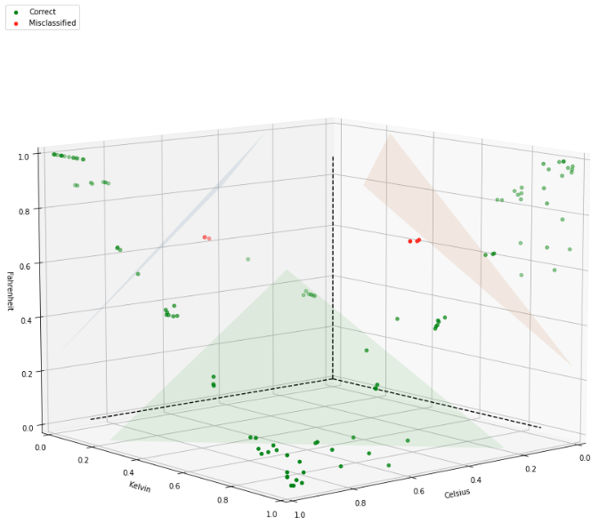
The core principle behind the inference algorithm is to compare the two distributions with the KS statistic. Since the unit of the reference distribution is known, we can convert this distribution into all three units (Celsius, Kelvin, and Fahrenheit), and compare the converted reference distribution with the measurement distribution. This yields a 3-dimensional point the unit square of KS statistics. For similar distributions, the KS statistic is close to zero, whereas for different distributions it approaches one. Hence, distributions with a distinguishable unit are located near the vertices (0, 1, 1), (1, 0, 1), and (1, 1, 0) in this unit square. By imposing geometrical constraints around the vertices, we can classify the points into Celsius, Kelvin, Fahrenheit, or Undecidable.
The Outcome: Unit Inference
In the figure below we see an example of implementing the above algorithm. Each point represents the three KS statistics computed under each null hypothesis. The axes represent the units under which the null hypothesis was formulated. The triangular plains divide the unit square into those four classes mentioned before. Correctly classified points are shown in green, whereas misclassified points are shown in red.
Conclusion
Our journey through hypothesis testing has taken us from concept to real-world application. It’s a method that allows us to make informed decisions and solve practical problems, like inferring temperature units from data. This tool is essential for anyone looking to make sense of the vast amounts of information in our digital world.
Are you ready to harness the power of hypothesis testing in your own projects? Whether you’re a data science enthusiast, a professional analyst, or simply curious about the world of statistics, the time to start is now. If you’ve found inspiration in these pages, don’t let it end here. Share your experiences, ask questions, in the comments below, and let’s continue the discussion.