From Data to Model Development: A Machine Learning Recipe for Detecting Outliers in Meteorological Data
In the ever-evolving field of meteorology, ensuring data quality is important. Machine learning (ML) offers innovative solutions to tackle complex challenges, such as detecting outliers in vast datasets. In this blog post, I’ll embark on a journey through the anatomy of a typical machine learning project. From defining the problem to developing the final model, we’ll break down the process into digestible chunks (I’ll mention briefly the deployment and monitoring steps of an ML project, but I won’t go into details in this blog). Then, we’ll dive deep into a real-world case study, showcasing how these steps were applied to detect collective outliers in air temperature measurements. Whether you’re a seasoned data scientist or just starting out, this post offers valuable insights into the intricacies of machine learning applied to meteorological data.
A Recipe of a Machine Learning Project: A High-Level Overview
Whenever you start working on an ML project think of it as making a meal. It’s a structured process that involves several key steps and each step is crucial to the project’s success. Here’s an overview of the typical stages:
-
Problem Definition – deciding the Menu
 : Before diving into data and algorithms (or pots and pans), it’s essential to clearly define the problem you’re trying to solve. What are the objectives? (What am I going to eat?) What type of problem is it (classification, regression, clustering, etc.)?
 -
Data Collection – grocery shopping
 : Once the problem is defined, the next step is to gather relevant data. This could involve collecting new data, using existing datasets, or a combination of both.
 -
Data Cleaning and Preprocessing – cleaning and peeling: Raw data is rarely ready for modeling. It often requires cleaning (handling missing values, removing outliers) and preprocessing (normalization, encoding categorical variables) to make it suitable for ML algorithms.
-
Feature Engineering – cutting, slicing, and mixing: This involves transforming the data to create features (input variables) that make the ML algorithm work better. It’s about representing the data in the best possible way.
-
Model Selection and Training – heat on
 and finally cooking
  : Choose an appropriate ML algorithm based on the problem type and data. Train the model using the processed data.
 -
Model Validation – tasting and smelling: After training, evaluate the model’s performance using appropriate metrics (accuracy, precision, recall, etc.). This helps in understanding how well the model is likely to perform on unseen data.
-
Hyperparameter Tuning and Final Evaluation – season, season, season… and taste
 : Most ML algorithms have hyperparameters that can be adjusted. Tuning them can lead to better model performance. At the end of the development process, the model is evaluated on a test set to estimate the performance of the model on unseen data.
 -
Deployment – serve it on the table: Once satisfied with the model’s performance, deploy it in a real-world setting. This could be on a server, in a cloud environment, or integrated into an application.
-
Monitoring and Maintenance – observe the yum yum
: Post-deployment, it’s essential to monitor the model’s performance and make necessary updates or retrain it as new data becomes available.
Hopefully, you now have a good sense of what it takes to successfully deliver – ehm cook – your first ML project. Now, let’s see how these steps manifest themself in a real-world scenario.
Detecting Collective Outliers in Air Temperature Measurements
Problem Definition
For the sake of illustrating the above steps, I going to present you a project I have been recently working on and have successfully delivered. In this project, the goal was to detect collective outliers of air temperature measurements, i.e., time series. You might wonder now what I mean by ‘collective’. Well, simply put it’s this:
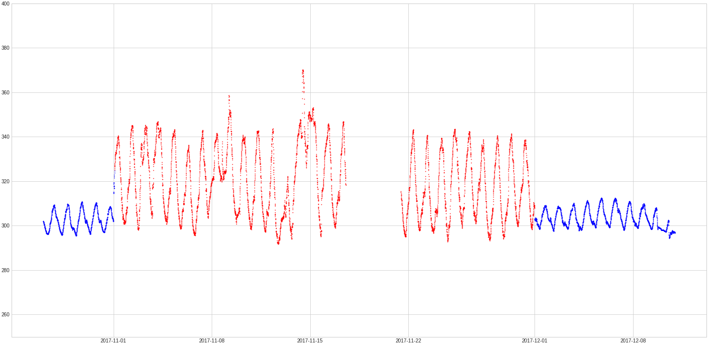 Slice of a time series showing ca. 6 weeks of air temperature measurements from a meteorological ground station. Blue and red points correspond to valid and invalid measurement records, respectively. The temperature is measured in Kelvin.
It’s not that important now to know the whole zoo of outliers (I might write a blog on various types of outliers in the future). All you need to be aware of is that these outliers are characterized by a continuous stream of abnormal values that only look abnormal from a global perspective, but locally look quite normal (if we ignore the values of the time series points). Given the nature of collective outliers, traditional supervised learning approaches, which rely on labeled data, were not suitable. The diverse shapes and durations of these outliers meant that there was no substantial labeled data available. Thus, the project leaned towards unsupervised models.
Data Collection
After we have a sense of what is the problem at hand we are ready to crunch some data. The first step consists of importing them. One of many Python libraries that can help us with doing exactly that is Pandas. This is how easily you can import a csv-file:
import pandas as pd
import numpy as np

data = pd.read_csv(
    path_data,                    # path to your data
    delimiter=';',                # the delimiter in the csv
    comment='#',                  # skips lines that star with '#'
    usecols=['datetime', 't'],    # selects columns in csv
    dtype={'t': 'float64'},       # defines the data type
    index_col='datetime',         # defines column for indexing
    parse_dates=True              # parses the dates in the index column
)

data.sort_index(inplace=True)     # chronologically sort the dates and times
data = data.asfreq('5min')        # samples data with uniform 5-min frequency
In most cases, it also works if you just specify the path and leave all other arguments as default values, and do the processing after the data are imported. Next, we need to prepare the imported data for our outlier detection model.
Data Cleaning, Preprocessing, and Feature Engineering
Raw data are raw, and no model can process any type of data out there in the wild. Hence, we need to prepare them for increasing the effectiveness of a model to do the job we want it to do. Data cleaning, data preprocessing, and feature engineering are the most important parts of any data science project where most time is spent. To detect a collection of successive outliers we need to prepare the data such that the model can process the data sequentially and the correlation in time of outliers is not destroyed. So, we split the data into segments of approximately 24 hours of data records (I have chosen to split the time series into daily segments as this is the smallest coherent periodicity of air temperature measurements).
sampling_frequency = 5

# number of timestamps covering 24 hours
day = 60 // sampling_frequency * 24

# nuber of days covering the whole time series
n_days = len(data) // day

# split series and put into segments
segments = np.array_split(data, n_days)
It is not so important that the segments are exactly of equal length as we are interested in extracting features that tell us something about the shape and the amplitude of daily air temperature measurements. One of the simplest ways of achieving that (and comes to mind to every physicist – including myself ![]() ) is through Fourier series coefficients. So, to capture this periodic nature and engineer features from the time series data, we apply the discrete Fourier transform (DFT) implemented in NumPy. To not consider noise in the data, we simply ignore higher frequencies by setting a cut-off N for the number of Fourier coefficients (here I am counting the number of coefficients in their Sine-Cosine form).
) is through Fourier series coefficients. So, to capture this periodic nature and engineer features from the time series data, we apply the discrete Fourier transform (DFT) implemented in NumPy. To not consider noise in the data, we simply ignore higher frequencies by setting a cut-off N for the number of Fourier coefficients (here I am counting the number of coefficients in their Sine-Cosine form).
# numpy.fft.rfft returns fourier coefficients of `time_domain_array`
# represented as complex numbers; fourier_coefficients contains
# the first `N` or `N` + 1  real-valued fourier coefficients
fourier_coefficients = np.fft.rfft(segment)[: (N + 2) // 2]

# break the complex fourier coefficients into real and imaginary
# components
fft_segment = np.stack(
    (fourier_coefficients.real[1:], fourier_coefficients.imag[1:]),
    axis=-1
).reshape(-1)

# insert the first real-valued fourier coefficient to the array
fft_segment = np.insert(fft_segment, 0, fourier_coefficients.real[0])

# if n_coefficients is even delete the last real-valued coefficient
# in `fft_segment`
if N % 2 == 0:
    fft_segment = np.delete(fft_segment, -1)
Each segment is now transformed into an N-dimensional Fourier space using the DFT.
Model Selection and Training
In this Fourier space, we are able to compare daily segments with each other based on their relative distance between each other. Points that are further away from a cluster of points are most probably representing segments of unusual shape and hence regarded as outliers. The Local Outlier Factor (LOF) from the scikit-learn library was chosen as the outlier detection method.
from sklearn.neighbors import LocalOutlierFactor

lof = LocalOutlierFactor(n_neighbors=n_neighbors)
lof.fit(fft_segments)

outlier_mask = lof.negative_outlier_factor_ < threshold
This algorithm returns a score that quantifies how much of an outlier a point is by comparing the density in its neighborhood of points with the density of all other points in the neighborhood. The size of the neighborhood is parameterized by n_neighbors. With a value for the threshold, we can then draw a decision boundary between the inliers and outliers. The choice of the optimal threshold value depends upon the type of error we want the LOF model to minimize. To get a quantitative sense of the model performance, we have a couple of performance metrics for classification problems – accuracy, precision, recall, etc.
Model Validation
The performance of the LOF model was evaluated based on precision, recall, and the F1-score on a separate hold-out set of time series datasets. The choice of the score had implications on the model’s ability to detect collective outliers. A precision-centric model was more conservative, detecting only the most evident outliers, while a recall-centric model could identify subtler outlier segments. The preference of one or another can then be used as a means of optimization.
Hyperparameter Tuning and Final Evaluation
To optimize the LOF model with respect to the hyperparameters (N, n_neighbors, threshold), a variant of grid-search and cross-validation was used (I’ll explain and show a hands-on application of scikit-learn’s grid search algorithm in a future blog). Instead of leaving out a subset of the training set for validation, subsets of datasets from various climatologic regions worldwide were left out. For example, if we have 25 datasets in total, then at the beginning of our ML project we put aside a few datasets for evaluation. Let’s say, we put aside 5 datasets – this constitutes our test set. The remaining 20 datasets are used for training, building data cleaning and preprocessing pipelines, and feature engineering. To optimize the hyperparameters, we then leave one dataset out (this is the hold-out set) from the set of 20 datasets and apply the outlier detection algorithm to the remaining 19 datasets. If we repeat this process for every dataset, we get a more robust estimate of the performance metric (either precision or recall) that is used for optimizing the LOF model. The hold-out set can be as large as half of the whole training set. If the training set is composed of diverse datasets, I would opt for smaller hold-out sets in favor of the robustness of the performance metrics, even though this increases the run-time of the grid-search algorithm.
Lessons Learned
The precision-recall trade-off is crucial in determining the model’s applicability. Depending on the desired outcome, one can opt for a fully automatic outlier detection pipeline or a semi-supervised approach involving human data quality control staff.
The project’s success also highlighted its potential applicability to other meteorological measurements. However, the periodic nature of temperature measurements offers an advantage, as a few leading Fourier coefficients can capture temperature oscillations. Other parameters, like relative humidity or wind speed, have more complex oscillations due to their variable nature.
Conclusion
Detecting collective outliers in meteorological data is a challenging yet crucial task. Through innovative feature engineering and the use of unsupervised learning techniques, this project showcased the potential of machine learning in ensuring data quality. As the field of meteorology continues to evolve, such methods will play an increasingly vital role in maintaining the integrity of our data.
Have you tackled similar challenges in your ML projects? Or perhaps you’ve used different techniques for outlier detection in meteorological data? I’d love to hear about your experiences and insights. Share your thoughts in the comments below, and let’s continue the discussion.